Self-Attention 4. Single-head Attention to Multi-head Attention
之前的所有流程可以被视为single-head attetnion流程.
First. stacking multiple single-header attention layer
实现multi-head attention的方式, 可以利用创建多个self-attention mechanism的方式, 每个mechanism有自己的weights, 然后我们组合他们的outputs.
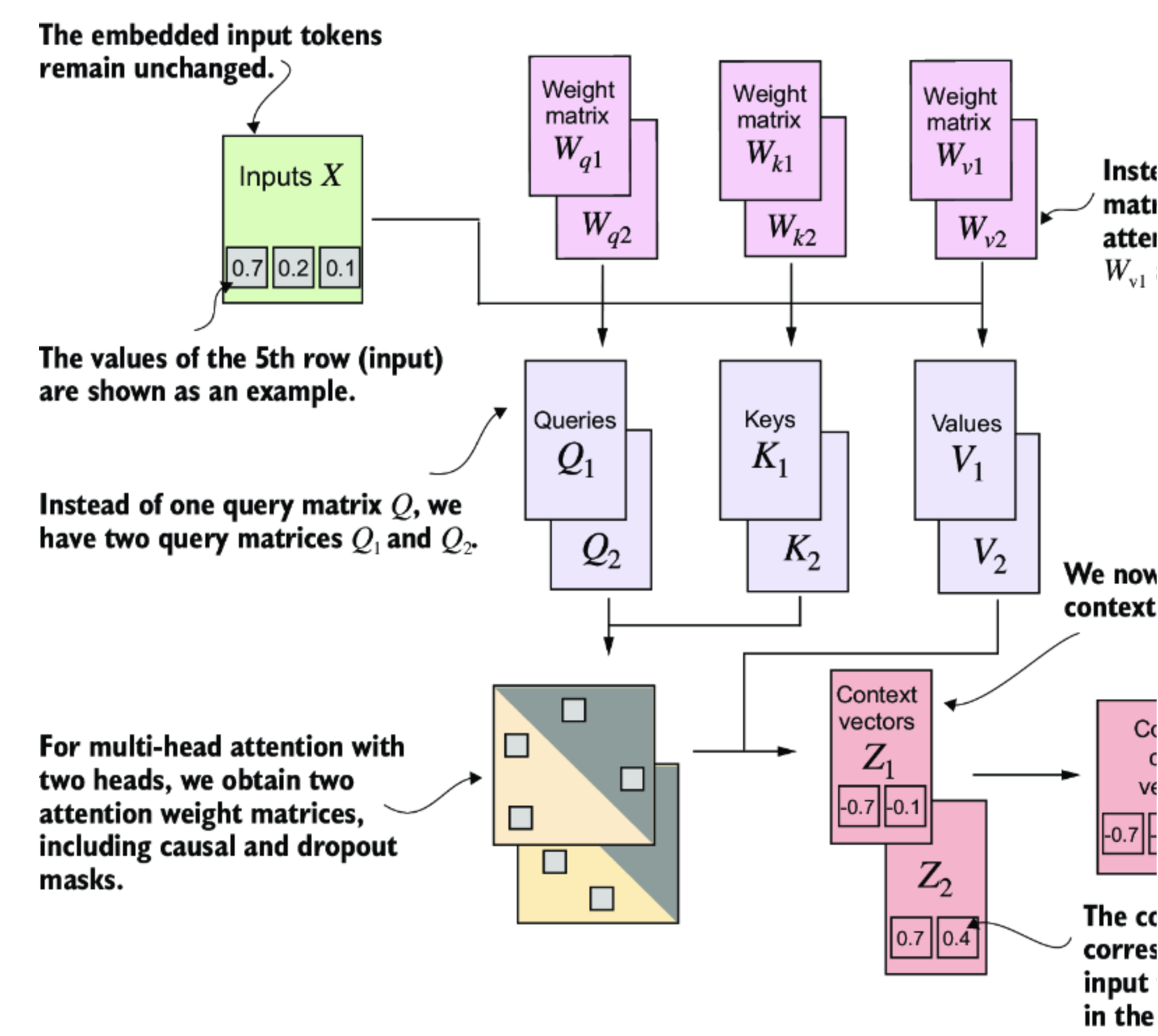
multi-head attention include two single-head attention
以上图例就是一个简单的multi-head attention, 由两个self-attention 堆叠而成.
multi-head attention的主要思想是使用不同的、学习到的线性投影多次(并行)运行self-attention mechanism——这是将输入数据(如注意力机制中的查询、键和值向量)与权重矩阵相乘的结果。
class MultiHeadAttentionWrapper(nn.Module):
  def __init__(self, d_in, d_out, context_length, dropout, num_heads, qkv_bias=False):
    super().__init__()
    self.heads = nn.ModuleList(
    [CausalAttention( d_in, d_out, context_length, dropout, qkv_bias )
    for _ in range(num_heads)]
    )
  def forward(self, x):
    return torch.cat([head(x) for head in self.heads], dim=-1)
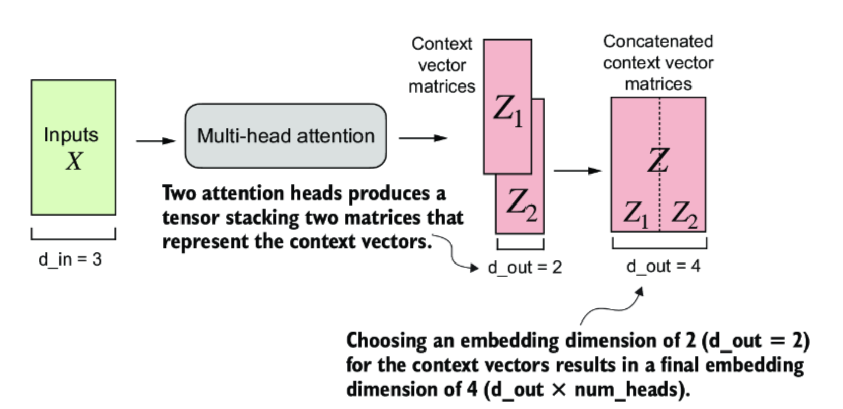
Two attention heads output
torch.manual_seed(123)
context_length = batch.shape[1] # This is the number of tokens
d_in, d_out = 3, 2
mha = MultiHeadAttentionWrapper( d_in, d_out, context_length, 0.0, num_heads=2 )
context_vecs = mha(batch)
print(context_vecs)
print("context_vecs.shape:", context_vecs.shape)

## result
tensor([[[-0.4519, 0.2216, 0.4772, 0.1063],
         [-0.5874, 0.0058, 0.5891, 0.3257],
         [-0.6300, -0.0632, 0.6202, 0.3860],
         [-0.5675, -0.0843, 0.5478, 0.3589],
         [-0.5526, -0.0981, 0.5321, 0.3428],
         [-0.5299, -0.1081, 0.5077, 0.3493]],

         [[-0.4519, 0.2216, 0.4772, 0.1063],
         [-0.5874, 0.0058, 0.5891, 0.3257],
         [-0.6300, -0.0632, 0.6202, 0.3860],
         [-0.5675, -0.0843, 0.5478, 0.3589],
         [-0.5526, -0.0981, 0.5321, 0.3428],
         [-0.5299, -0.1081, 0.5077, 0.3493]]], grad_fn=<CatBackward0>) context_vecs.shape: torch.Size([2, 6, 4])
结果 context_vecs 张量的第一个维度是 2,因为我们有两个输入文本(输入文本是重复的,这就是这些上下文向量完全相同的原因)。第二个维度指的是每个输入中的 6 个标记。第三个维度指的是每个标记的四维嵌入。
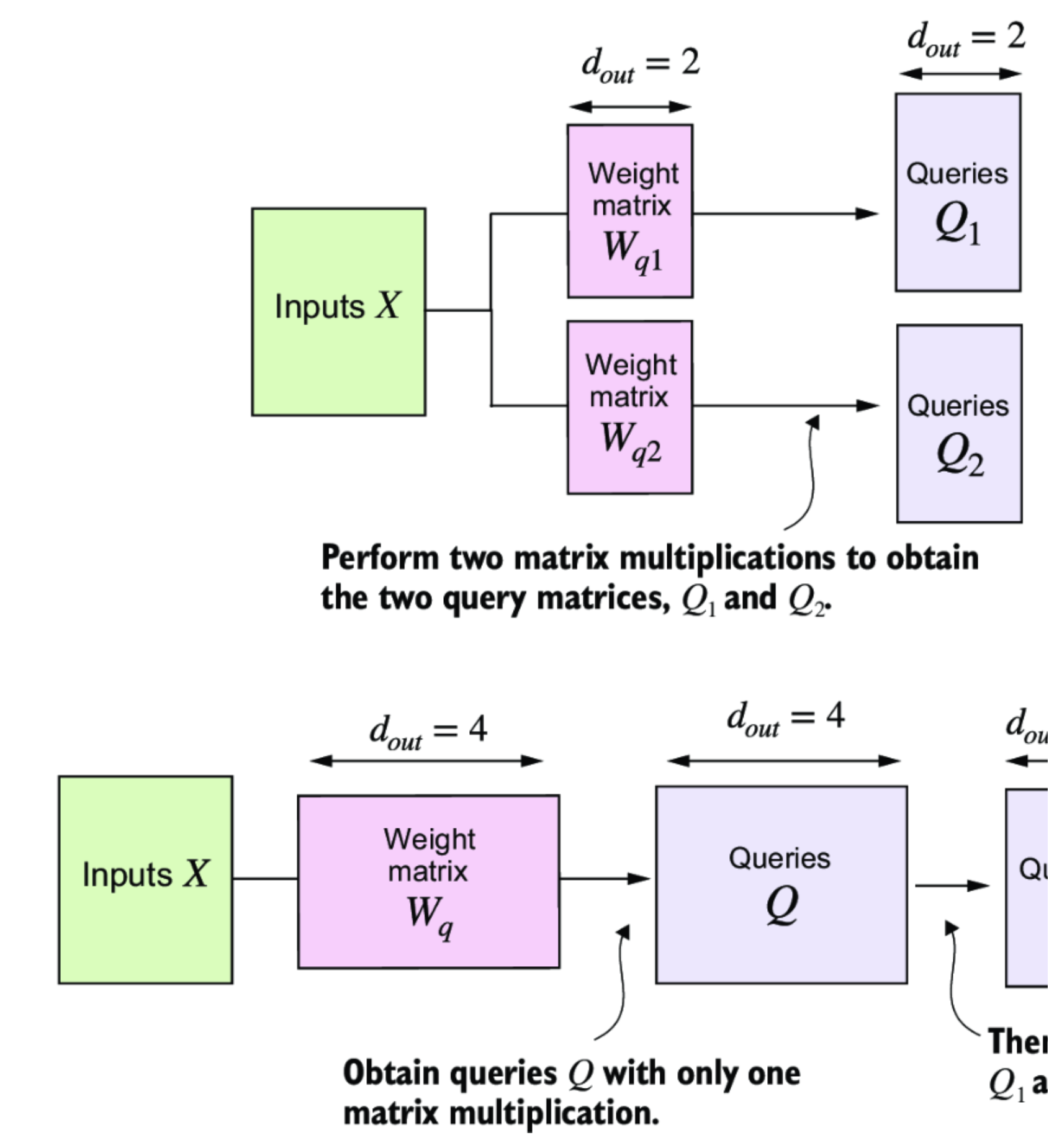
Second. implementing multi-head attention with weight splits
我们有了MultiHeaderAttentionWrapper和CasualAttention, 融合一下变成MultiHeadAttention
class MultiHeadAttention(nn.Module):
    def __init__(self, d_in, d_out, context_length, dropout, num_heads, qkv_bias=False):
        super().__init__()
        assert (d_out % num_heads == 0), "d_out must be divisible by num_heads"

        self.d_out = d_out
        self.num_heads = num_heads
        self.head_dim = d_out // num_heads  # 1

        self.W_query = nn.Linear(d_in, d_out, bias=qkv_bias)
        self.W_key = nn.Linear(d_in, d_out, bias=qkv_bias)
        self.W_value = nn.Linear(d_in, d_out, bias=qkv_bias)
        self.out_proj = nn.Linear(d_out, d_out)  # 2
        self.dropout = nn.Dropout(dropout)

        self.register_buffer(
            "mask", torch.triu(torch.ones(context_length, context_length), diagonal=1)
        )

    def forward(self, x):
        b, num_tokens, d_in = x.shape

        keys = self.W_key(x)  # 3
        queries = self.W_query(x)  # 3
        values = self.W_value(x)  # 3

        keys = keys.view(b, num_tokens, self.num_heads, self.head_dim)  # 4
        values = values.view(b, num_tokens, self.num_heads, self.head_dim)  # 4
        queries = queries.view(b, num_tokens, self.num_heads, self.head_dim)

        keys = keys.transpose(1, 2)  # 5
        queries = queries.transpose(1, 2)  # 5
        values = values.transpose(1, 2)  # 5

        attn_scores = queries @ keys.transpose(2, 3)  # 6

        mask_bool = self.mask.bool()[:num_tokens, :num_tokens]  # 7
        attn_scores.masked_fill_(mask_bool, -torch.inf)  # 8
        attn_weights = torch.softmax(attn_scores / keys.shape[-1]**0.5, dim=-1)
        attn_weights = self.dropout(attn_weights)

        context_vec = (attn_weights @ values).transpose(1, 2)  # 9 # 10
        context_vec = context_vec.contiguous().view(b, num_tokens, self.d_out)

        context_vec = self.out_proj(context_vec)  # 11
        return context_vec
[!NOTE]
- 将投影维度减少到与所需输出维度匹配
- 使用线性层组合单注意力机制输出
- 张量变形(Tensor shape): (b, numtokens, dout)
- 我们通过添加 numheads 维度隐式地拆分矩阵。然后我们展开最后一个维度: (b, numtokens, dout) -> (b, numtokens, numheads, headdim)。
- 从 shape (b, numtokens, numheads, headdim) 转置为 (b, numheads, numtokens, headdim)
- 计算每个头的点积
- 将掩码截断到标记数量
- 使用掩码填充注意力分数
- 张量变形(Tensor shape): (b, numtokens, nheads, head_dim)
- 组合头部,其中 self.dout = self.numheads * self.head_dim
- 添加一个可选的线性投影
CleanShot 2024-11-13 at 11.54.08@2x.png
为说明这一批量矩阵乘法,假设我们有以下张量:
The shape of this tensor is (b, numheads, numtokens, head_dim) = (1, 2, 3, 4).
a = torch.tensor([[[[0.2745, 0.6584, 0.2775, 0.8573],  #1
                    [0.8993, 0.0390, 0.9268, 0.7388],
                    [0.7179, 0.7058, 0.9156, 0.4340]],
                    [[0.0772, 0.3565, 0.1479, 0.5331],
                    [0.4066, 0.2318, 0.4545, 0.9737],
                    [0.4606, 0.5159, 0.4220, 0.5786]]]])
现在我们在张量本身和张量的一个视图之间执行批量矩阵乘法。我们转置了最后两个维度,numtokens 和 headdim:
print(a @ a.transpose(2, 3))

tensor([[[[1.3208, 1.1631, 1.2879],
          [1.1631, 2.2150, 1.8424],
          [1.2879, 1.8424, 2.0402]],
          [[0.4391, 0.7003, 0.5903],
          [0.7003, 1.3737, 1.0620],
          [0.5903, 1.0620, 0.9912]]]])
在这种情况下,PyTorch中的矩阵乘法实现处理四维输入张量,以便在最后两个维度(numtokens,headdim)之间进行矩阵乘法,然后为各个head重复这一操作。
例如,上述方式变成了计算每个头的矩阵乘法的更简洁方法:
first_head = a[0, 0, :, :]
first_res = first_head @ first_head.T
print("First head:\n", first_res)

second_head = a[0, 1, :, :]
second_res = second_head @ second_head.T
print("\nSecond head:\\n", second_res)

# 结果与print(a @ a.transpose(2, 3)) 一致
First head:
tensor([[1.3208, 1.1631, 1.2879],
        [1.1631, 2.2150, 1.8424],
        [1.2879, 1.8424, 2.0402]])

Second head:
tensor([[0.4391, 0.7003, 0.5903],
        [0.7003, 1.3737, 1.0620],
        [0.5903, 1.0620, 0.9912]])
继续讨论多头注意力,在计算出注意力权重和上下文向量后,所有头的上下文向量被转置回形状 (b, numtokens, numheads, headdim)。然后,这些向量被重新形状化(拉平)为形状 (b, numtokens, d_out),有效地结合了来自所有头的输出。
此外,我们在组合头部之后向MultiHeadAttention添加了一个输出投影层(self.out_proj),而CausalAttention类中并不存在此层。这个输出投影层并不是严格必要的,但在许多大型语言模型架构中常常使用,因此我在这里添加它以保证完整性。
torch.manual_seed(123)
batch_size, context_length, d_in = batch.shape
d_out = 2
mha = MultiHeadAttention(d_in, d_out, context_length, 0.0, num_heads=2)
context_vecs = mha(batch)
print(context_vecs)
print("context_vecs.shape:", context_vecs.shape)

# result
tensor([[[0.3190, 0.4858],
         [0.2943, 0.3897],
         [0.2856, 0.3593],
         [0.2693, 0.3873],
         [0.2639, 0.3928],
         [0.2575, 0.4028]],

         [[0.3190, 0.4858],
         [0.2943, 0.3897],
         [0.2856, 0.3593],
         [0.2693, 0.3873],
         [0.2639, 0.3928],
         [0.2575, 0.4028]]], grad_fn=<ViewBackward0>)

context_vecs.shape: torch.Size([2, 6, 2])
作为对比,最小的GPT-2模型(1.17亿参数)有12个注意力头,上下文向量嵌入大小为768。最大的GPT-2模型(15亿参数)有25个注意力头,上下文向量嵌入大小为1,600。在GPT模型中,令牌输入和上下文嵌入的嵌入大小是相同的(din = dout)。